This is the second installment to my series on machine learning, which builds on my initial post on neural networks “Bridging the gap between neural networks and functions”. In this post, we’ll explore how scaling up dot product operations using matrix multiplication enables modern machine learning. As with the rest of this series, we’ll keep the explanations intuitive yet detailed, aiming to help software engineers build a foundation for understanding.

I’m aiming to make these posts accessible to other software engineers, by giving explanations that are grounded in ways that should be familiar to us, but which don’t assume a lot of prior knowledge. I’m not an expert in this field, so please let me know if you notice any inaccuracies or have any feedback by dropping me an email.

In my first post, the forward pass of a neuron was described as computing the weighted sum of inputs plus a bias followed by a non-linear activation function. Some simple psuedocode was used to show this:

js
activation(add(sum(multiply(weights, inputs)), bias));

In reality, instead of computing the “weighted sum of inputs” using sum(multiply(weights, inputs)) (e.g. $\text{{activation}}\left(\sum_i w_i \cdot x_i + b\right)$) we use a mathematical operation called the dot product (e.g. $\text{{activation}}\left(W \cdot x + b\right)$).

To implement this we can take two vectors represented by arrays of equal length, zip them together, multiply each pair, and then sum these products to produce a single number.

e.g.

typescript
// This is a highly inefficient implementation of "dot product"
// and the code only exists to provide an intuitive explanation
// of how it works.
//
// See: https://github.com/Jam3/math-as-code#dot-product
function dotProduct(v1: number[], v2: number[]): number {
  return sum(zip(v1, v2).map(([x, y]) => x * y));
}
 
function zip<T, U>(a: T[], b: U[]): [T, U][] {
  if (a.length !== b.length) {
    throw new Error("Arrays must have the same length");
  }
 
  return a.map((x, i) => [x, b[i]]);
}
 
function sum(arr: number[]): number {
  return arr.reduce((acc, val) => acc + val, 0);
}
 
const weights = [1, 2, 3];
const inputs = [4, 5, 6];
 
const weightedSum = dotProduct(weights, inputs); // 32

Vector representations

A vector is a representation of a multi-dimensional quantity with a magnitude and direction. It can be thought of as an arrow starting from the origin of the coordinate system $(0, 0, 0, ...)$ and ending at a point in vector space $(x, y, z, ...)$.

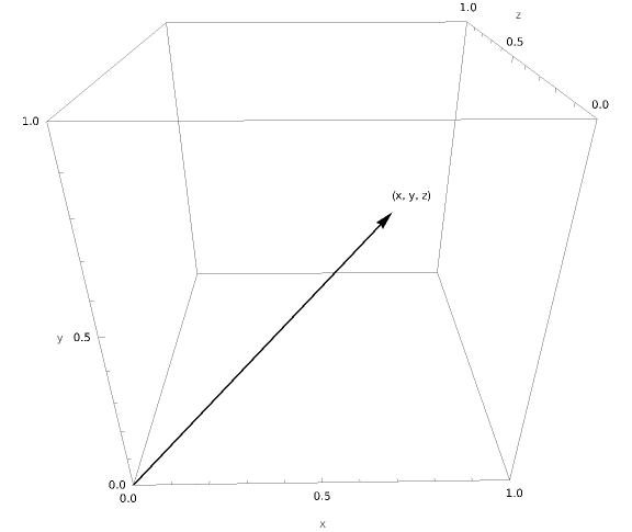
For example, in the code above, the weights vector [1, 2, 3] can be thought of as an arrow starting from the origin of the coordinate system $(0, 0, 0)$ and ending at the point $(1, 2, 3)$, while the inputs vector [4, 5, 6] can be thought of as an arrow starting from the origin of the coordinate system $(0, 0, 0)$ and ending at the point $(4, 5, 6)$.

In machine learning, we often use vectors to represent the individual input rows of a dataset, where each dimension of a vector is a column representing an attribute/feature of an input row (e.g. $(f_1, f_2, f_3, ..., f_n)$). For example, if we were trying to predict the price of a house, we might have a dataset in which each row was a vector representing a house with the following numeric features: number of bedrooms, number of bathrooms, square footage, number of floors, and so on.

We can also use vectors to represent non-numeric data, however, in order to do this, we need to encode this data into a numeric representation. For instance, categorical variables (e.g. $colors = \{\mathit{red}, \mathit{blue}, \mathit{green}\}$ or $countries = \{\mathit{USA}, \mathit{UK}, \mathit{Canada}\}$) can be represented using a “one-hot” encoded vector (e.g. $(0, 0, 1, 0, ..., 0)$) by first assigning each category a unique integer and then setting all elements of the vector that we want to represent this category to $0$ except for the element at the index of the unique integer we assigned to the category (which we’d set to $1$).

In language models, the “one-hot” encoding approach to representing non-numeric data falls short as it does not capture any information about the semantic relationship between words. For example, the words “dog” and “cat” are more similar to each other than they are to the word “democracy”, but this is not reflected in the one-hot vectors for these words. Word embeddings, learned from a large amount of text data, solve this problem by embedding words in a continuous vector space where similar words are placed closer together. For example, in this space, the word “dog” might be represented as $(0.9, -0.2, 0.4, ...)$ and “cat” might be $(0.8, -0.3, 0.5, ...)$. This information can be learned due to the “distributional hypothesis” which states that words that frequently occur close together tend to have similar meanings.

“You shall know a word by the company it keeps.”

— J.R. Firth

Originally these embeddings were learned using specific algorithms such as Word2Vec and GloVe, however in transformer-based models like GPT, these embeddings can be learned during the training process via backpropagation and through their interactions within the self-attention mechanism.

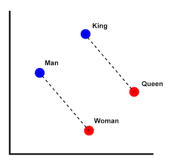
The capacity to capture the semantic relationships between words is the essence of why “word embeddings” are able to represent words. And, they are in fact, so effective at achieving this that not only do they allow us to see similarities between words, but they also enable us to perform arithmetic operations on these; a classic example being $king - man + woman ≈ queen$.

Semantic arithmetic is more than just a novelty — it’s consequential and carries significant implications. It means that the vector space is a semantic space that captures meaning itself. This semantic space can provide a kind of substrate for models to operate on allowing for (1) small iterative arithmetic adjustments to reflect nuanced changes in meaning, (2) avoidance of discontinuities in meaning and possibility of interpolated or intermediate meanings during computation, and (3) representation of the nameless or even ineffable.

Dimensionality

Dimensionality refers to the number of attributes or features that belong to each data point (row/vector) of a dataset.

In practice, the vectors used in machine learning can have an overwhelmingly large number of dimensions. For instance, a word embedding in GPT-3 has 768 dimensions. Because of this, in order to make sense of them, we often have to resort to dimensionality reduction techniques like PCA, t-SNE, or UMAP. These techniques map high-dimensional data into a lower-dimensional space, typically 2 or 3 dimensions, while attempting to preserve as much of the data’s original structure and information as possible. This helps us to visualize the data to unveil patterns or relationships within it.

For example, if we ran a dimensionality reduction algorithm on the word embeddings of the words “dog”, “cat” and “democracy” and plotted these on a graph, we might see something like this:

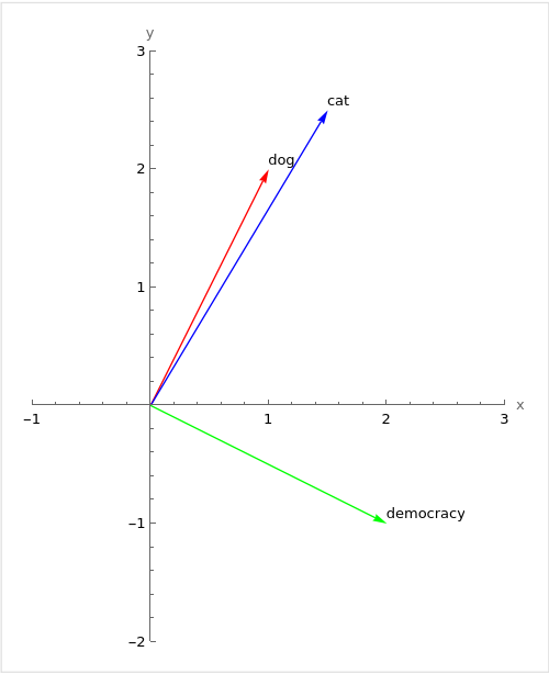
Dimensionality reduction does lead to some information loss and isn’t perfect but it can be very useful when dealing with high-dimensional data that otherwise would be practically impossible to interpret.

Computing similarity

Of course, we don’t want to resort to drawing a graph every time we wish to compare two vectors. Instead, we employ a similarity metric to measure the similarity between two vectors. One such metric is the dot product operation described at the beginning of this post.

As a metric of similarity, the dot product has some useful properties. For example, if two vectors are pointing in the same direction, the dot product between them will be positive suggesting they are similar. If they are pointing in opposite directions, the dot product will be negative suggesting they are dissimilar. And, if they are perpendicular to each other, the dot product will be zero — indicating orthogonality and suggesting that the two vectors are independent from each other or capturing different information within the vector space.

Crucially, the dot product’s measure of similarity is sensitive to both the direction and magnitude of the vectors. For example, if we were to double the overall magnitude of the vector for “cat” in the above diagram, the dot product between it and the vector for “dog” would increase even though the two vectors are still pointing in the same direction and therefore the words are just as similar to each other as they were before. This may or may not be desirable depending on the task at hand — if we want a measure of similarity that is less sensitive to the magnitude of the vectors, we can utilize cosine similarity or a scaling factor.

Note that, in high-dimensional spaces, the interpretation of the dot product becomes less straightforward as negative dot products could indicate that the vectors are spread apart in the vector space instead of being opposite or dissimilar to each other; this similarly affects both zero and positive dot products.

Parallelising dot products: matmul goes brrr

The dot product shows up again and again in machine learning. It’s used in the forward pass of neural network neurons to compute “weighted sums of inputs”, in dot product similarities within attention mechanisms, and even has a hashmap-like usage in which one-hot encoded vectors are used for lookups.

It’s often quipped that modern machine learning boils down to performing matrix multiplications as quickly as possible and then stacking more and more layers of these until the network is able to generalize. There’s more than a grain of truth here. The ability to quickly process an incredible amount of dot product operations is key to training models like GPT-3 as these require a massive amount of computational power (in the ballpark of $3.14 \times 10^{23}$ FLOPS were required to train GPT-3).

Fortunately, in the last few decades there has been a lot of investment into the efficient execution of floating point calculations, driven primarily by the demand for high-quality visuals in videogames. The architecture of GPUs allow them to perform many similar operations simultaneously, and this hardware and algorithmic investment has ended up delivering a bit of a windfall for AI, as they were able to be repurposed for machine learning. They now form the backbone of modern machine learning computation. (Although there are also other architectures being developed for this purpose which harness systolic arrays and attempt to directly optimize for the repeated multiply-accumulate operations (MAC) that constitute dot product operations).

In order to take advantage of the parallelism offered by GPUs, we need to be able to represent our data as matrices. A matrix is a two-dimensional array of numbers, and can be thought of as a collection of vectors, and roughly analogous to a spreadsheet or table of rows. Matrices are stored in contiguous blocks of memory (known as contiguous memory layouts), which helps to speed up data loading and processing due to locality of reference. Matrices also enable further optimizations to be made to their operations using techniques like matrix tiling and by vectorizing calculations using single instruction, multiple data (SIMD) instructions.

In graphics programming, matrices are a way to combine linear transformations (scale, rotation, translation, etc) into a single structure so we can apply these transformations onto vectors.

In contrast, in machine learning, we frequently use matrices for their ability to parallelize dot product operations (with matrix multiplication) or to parallelize other element-wise floating point vector operations like addition and subtraction. For example, rather than computing the forward pass of a single neuron one at a time (e.g. activation(add(dotProduct(weights, inputs), bias))), we can compute the forward pass of an entire layer of neurons in parallel by representing the weights of the layer as a matrix (e.g. activation(add(matmul(weightsByNeuron, inputs), biasByNeuron))), where each row of the weightsByNeuron matrix represents a neuron and each column represents a weight for a particular input. This allows us to compute the dot product (“weighted sum”) of each row of this matrix with the inputs in parallel.

Matrix multiplication (e.g. matmul) is an operation from linear algebra that has both a procedural and geometric interpretation:

• Procedurally, it allows us to compute the dot product of each row of the first matrix with each column of the second matrix. In a nutshell: each cell in the resulting matrix is a measure of how closely the row from the first matrix matches the column from the second matrix (in terms of their dot product).
• Geometrically, it is like composing two linear transformations (e.g. scaling, rotating, skewing, or shearing the space) to create a new transformation that combines these.

To better understand these two interpretations, André Staltz has an interactive visualization showing how a matrix multiplication operation is calculated, while 3Blue1Brown has a great video explaining the operation in terms of geometry, by showing how a matrix can represent the transformation of a vector space into a new coordinate system.

It’s defined like so:

Matrix multiplication operations are not allowed unless the number of columns in the first matrix $A$ matches the number of rows in the second matrix $B$. The resulting matrix $C_{\textcolor{red}{a},\textcolor{blue}{b}}$ will then have dimensions determined by the remaining dimensions of the input matrices.

An inefficient but simple implementation of matmul might look like this:

typescript
// This is an incredibly inefficient implementation of "matrix multiplication"
// and the code only exists to provide an intuitive explanation of how it
// works.
//
// If you want a faster implementation, you should use `PyTorch` which is
// already very optimized or if you'd like to learn how GPUs work try to
// reimplement the logic below using WebGPU using the techniques
// described here: https://jott.live/markdown/webgpu_safari
function matmul(A: number[][], B: number[][]): number[][] {
  if (A[0].length !== B.length) {
    throw new Error(
      `The number of columns in A must equal the number of rows in B: ` +
        `${A[0].length} !== ${B.length}`
    );
  }
 
  const aRows = A.length;
  const bCols = B[0].length;
  const sDims = A[0].length;
  const C = Array.from({ length: aRows }).map(() =>
    Array.from<number>({ length: bCols }).fill(0)
  );
 
  // For s from 0 to sDims, accumulate A[a][s] times B[s][b].
  for (let a = 0; a < aRows; a++) {
    for (let b = 0; b < bCols; b++) {
      for (let s = 0; s < sDims; s++) {
        C[a][b] += A[a][s] * B[s][b];
      }
    }
  }
 
  return C;
}
 
const A = [
  [1, 2, 3],
  [4, 5, 6],
];
const B = [
  [7, 8],
  [9, 10],
  [11, 12],
];
 
const C = matmul(A, B);
// [
//   [58, 64],
//   [139, 154]
// ]

🔑🔑🔑

In “bridging the gap between neural networks and functions”, we argued that essential to the use of backpropagation was that all inputs must be real-valued numeric values and all operations must be differentiable and composable. As we’ve shown, word embeddings are real-valued numeric vectors, and matrix multiplication operations are differentiable and composable due to being made up of many dot product operations that are ultimately composed of many multiply-accumulate (MAC) operations.

As a software engineer, the matrix multiplication convention of multiplying the columns of one matrix by the rows of another matrix seems arbitrary and confusing. As far as I can understand, it comes from the geometric interpretation of matrix multiplication as composing linear transformations (e.g. scaling, rotating, skewing, or shearing the space). While in machine learning we seem to primarily use matrix multiplication for its ability to parallelize dot product operations, it’s possible that the kind of semantic arithmetic mentioned earlier when discussing word embeddings makes it reasonable to interpret matrix multiplication within high-dimensional vector spaces geometrically. We know that these models do sometimes appear to perform geometric operations in order to compute outputs, for example, in “Progress measures for grokking via mechanistic interpretability” a simple transformer was trained to perform modular addition (aka, “clock” arithmetic) and when the authors reverse-engineered the algorithm learned by the network they found that it was using discrete Fourier transforms and trigonometric identities to convert addition to rotation about a circle. If your whole world consists of distances in high-dimensional vector spaces perhaps it makes sense that the way you compute outputs will be composed of angles and frequencies.

What is abundantly clear is that modern machine learning models are highly demanding of computational resources (FLOPS) and that matrix multiplication operations can concisely express the application of parallel dot product operations in equations.

So, to conclude: dot products are found at the heart of many operations in machine learning. They are integral for calculating weighted sums, measuring similarity, and even power the “attention” mechanism in transformers. However, their real power comes when we scale up the number of these operations using matrix multiplication and as a consequence cause complex linear transformations within high-dimensional spaces. GPUs are instrumental to this, efficiently handling the massive computational demands it requires, and we have videogames to thank for this!